Introduction

Overview

Teaching: 15 min
Exercises: 0 min

Questions

• How is OpenRefine useful?

Objectives

• Describe OpenRefine’s uses and applications.

• Differentiate data cleaning from data organisation.

• Experiment with OpenRefine’s user interface.

• Locate helpful resources to learn more about OpenRefine.

What is OpenRefine?

OpenRefine is a powerful tool for working with messy data: cleaning it; transforming it from one format into another. It provides tools that allow to understand even large data sets, and allows you to get a feel of the “shape” and content of the data. This helps inform the direction of your later analysis of the data.

It runs in a browser, which might lead you to think that it’s a Web or Cloud program. It is not! It is a desktop Java application that uses a browser as a convenient interface. No internet connection is needed, and none of your data will be sent to a remote server.

OpenRefine does not modify your original dataset. It stores your raw data set, and presents views on that data set after applying the data cleaning steps you specify. This means you never lose your original data and you can easily undo changes. OpenRefine saves as you go, so you can return to the project at any time and pick up where you left off. It allows you to save the raw data, processed data and all of the data cleaning steps in a file. It also allows you to export only your processed data to a new file.

OpenRefine is:

• free
• open source (source on GitHub)
• has a large growing community, from novice to expert, ready to help
• works with large-ish datasets (100,000s rows), but does not yet scale to many millions of rows.

Why do we need a tool like OpenRefine?

It is important to know what how your data is transformed as you move from data collection to data analysis. Sometimes you need to clean your data before you can analyse it. If you don’t keep a record of how you clean the data, you will not be able to reproduce your results - and this is vital if you want to demonstrate how a result was generated or repeat the analysis later. Reproducibility is becoming increasingly important for journals, funders and other institutions. If you can demonstrate every step in your data cleaning and analysis, it is likely to become increasingly difficult to publish results or win funding.

Manually documenting every data cleaning step is laborious and error prone. With OpenRefine, you can capture every step automatically, and then easily share the process with collaborators. In addition:

• OpenRefine provides tools that make data cleaning more straightforward, which saves a lot of time.
• It makes powerful but complex processes, such as clustering algorithms, easy to use.
• Any operation in OpenRefine can be easily reversed or undone.
• It is straightforward to repeat a data cleaning process across multiple files - saving even more time.

Where to find help and further reading

You can find out more on the OpenRefine website and check out some great introductory videos. There is a Google Group that can answer a lot of beginner questions and problems. OpenRefine recipes, scripts, projects, and extensions are available too, where you can find useful transformations to run on your own data.

The OpenRefine GitHub wiki page has a reference of the General Refine Expression Language (GREL) used by OpenRefine. We won’t be covering GREL in this lesson but it is a powerful scripting language that is worth learning once you get the hang of OpenRefine as it will enable you to do even more complex data cleaning and transformation steps.

Click the arrow in the bottom right of the page to proceed to the next episode.

Key Points

• OpenRefine is a powerful and free, open source tool that can be used for data cleaning.

• OpenRefine will automatically track any steps you take in working with your data, and will leave your original data intact.

Opening and Exploring Data

Overview

Teaching: 20 min
Exercises: 15 min

Questions

• How can we import our data into OpenRefine?

• How can we summarise our data?

• How can we find errors in our data?

• How can we edit data to fix errors?

• How can we convert column data from one data type to another?

Objectives

• Create a new OpenRefine project from a CSV file.

• Learn about different types of facets and how they can be used to summarise data of different data types.

Creating a project

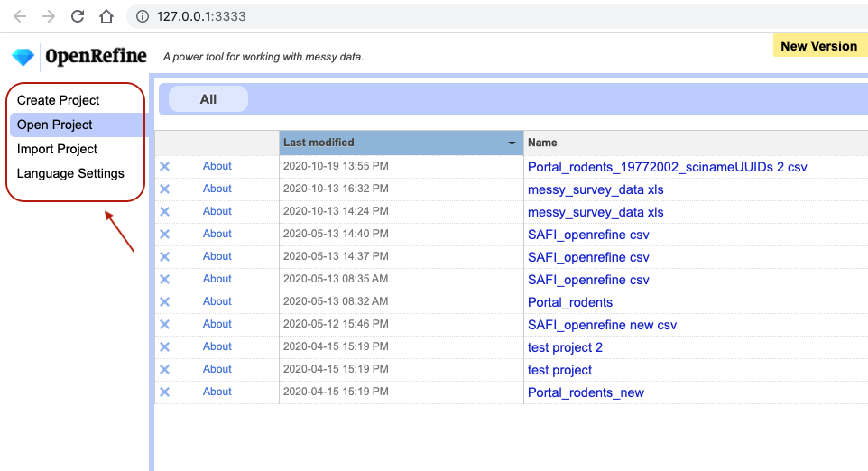
Start OpenRefine, which will open in your browser (at the address http://127.0.0.0:3333). Once OpenRefine is launched in your browser, the left margin has options to Create Project, Open Project, or Import Project. Here we will create a new project and import our portal rodents data.

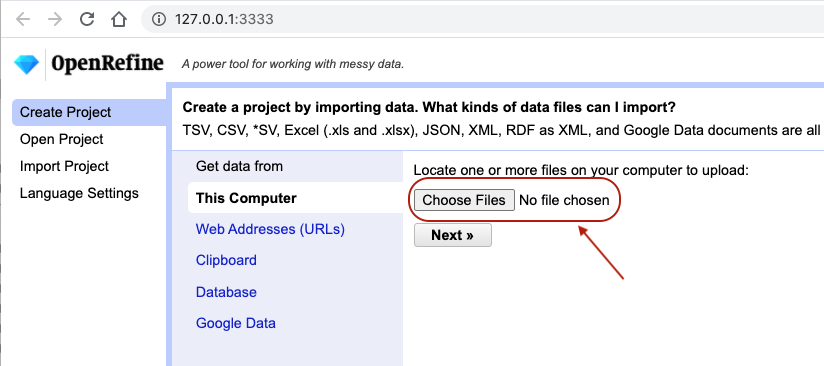
1. Click Create Project from the left margin and select then This Computer (because you’re uploading data from your computer).
2. Click Choose Files and browse to where you stored the file Portal_rodents_19772002_scinameUUIDs.csv. Select the file and click Open, or just double-click on the filename.
3. Click Next>> under the browse button to upload the data into OpenRefine.

4. On the next screen, OpenRefine will present you with a preview of your data. You can check here for obvious errors, if, for example, your file was tab-delimited rather than comma-delimited, the preview would look strange (and you could correct it by choosing the correct separator and clicking the Update Preview button on the right. If you selected the wrong file, click <<Start Over at the top left.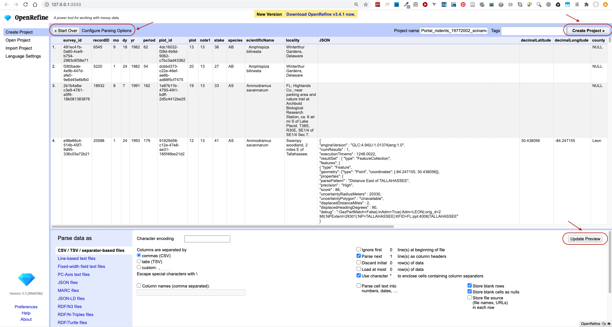

   

5. In the middle of the page, will be a set of options (Character encoding, etc.). Make sure the tick box next to Trim leading & trailing whitespace from strings is not ticked. (We’re going to need the leading whitespace in one of our examples.)
6. If all looks well, click Create Project>> in the top right. You will be presented with a view onto your data. This is OpenRefine!

Let’s now start exploring and getting a higher-level overview of our data - summarising and looking for potential outliers and errors.

Data file types supported

OpenRefine can import a variety of different file types, including tab separated (tsv), comma separated (csv), Excel (xls, xlsx), JSON, XML, RDF as XML, and Google Spreadsheets. See the OpenRefine Importers page for more information.

Data faceting

Facets are one of the most useful features of OpenRefine. Data faceting is a process of exploring data by applying multiple filters to investigate its composition. It also allows you to identify a subset of data that you wish to change in bulk.

OpenRefine Wiki: Faceting

Full documentation on faceting can be found at OpenRefine Wiki: Faceting

OpenRefine supports a range of facets, including:

• Text facet for working with textual data,
• Numeric and Scatterplot facets for working with numeric data,
• Timeline facet for working with dates, and
• number of customized facets (some of which we will cover shortly).

Text facet

A ‘text facet’ groups all the identical text values in a column and lists each value with the number of records in which it appears. The facet information always appears in the left hand panel in the OpenRefine interface. We will use text faceting to look for potential errors in the scientificName column.

1. Click the down arrow next to the scientificName column.
2. Choose Facet > Text facet.

3. In the left panel, you’ll now see a box containing every unique value in the scientificName column along with a number representing how many times that value occurs in the column.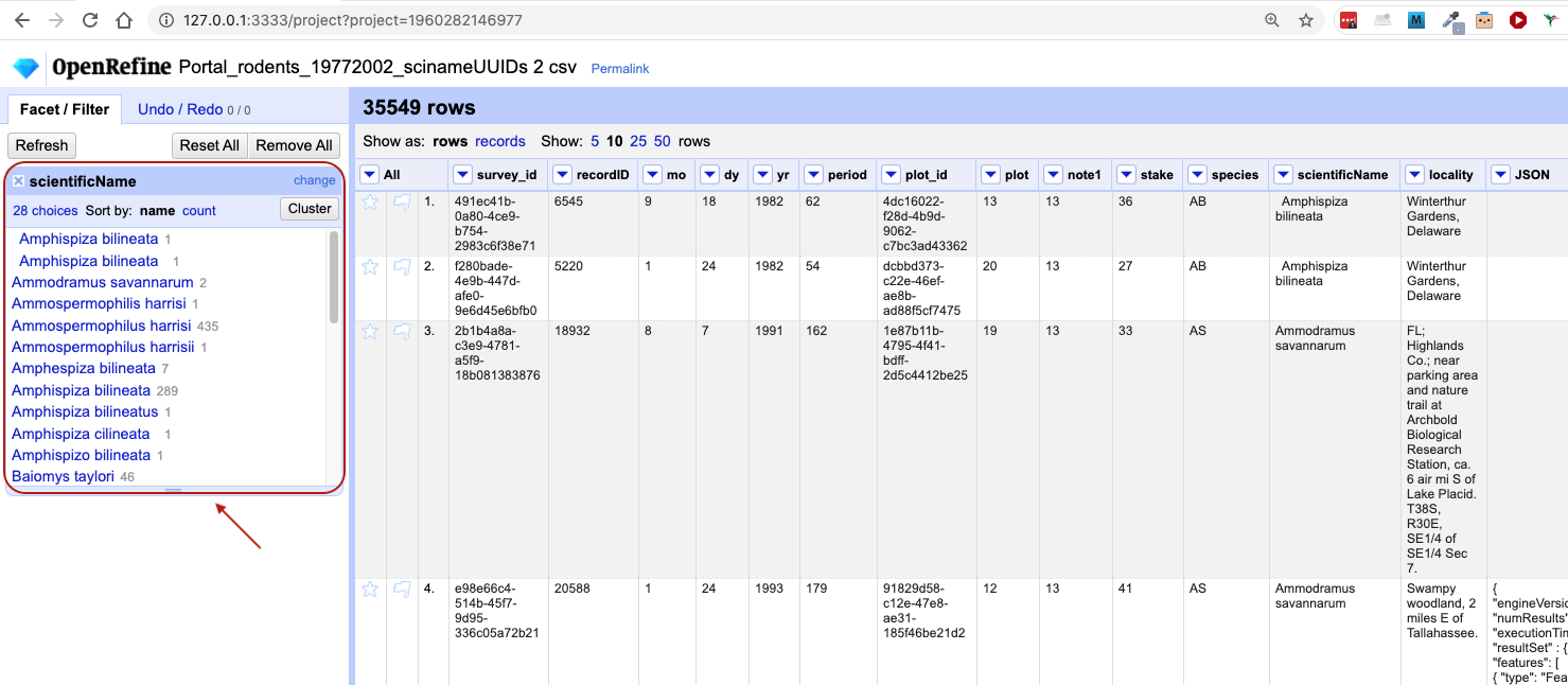

   

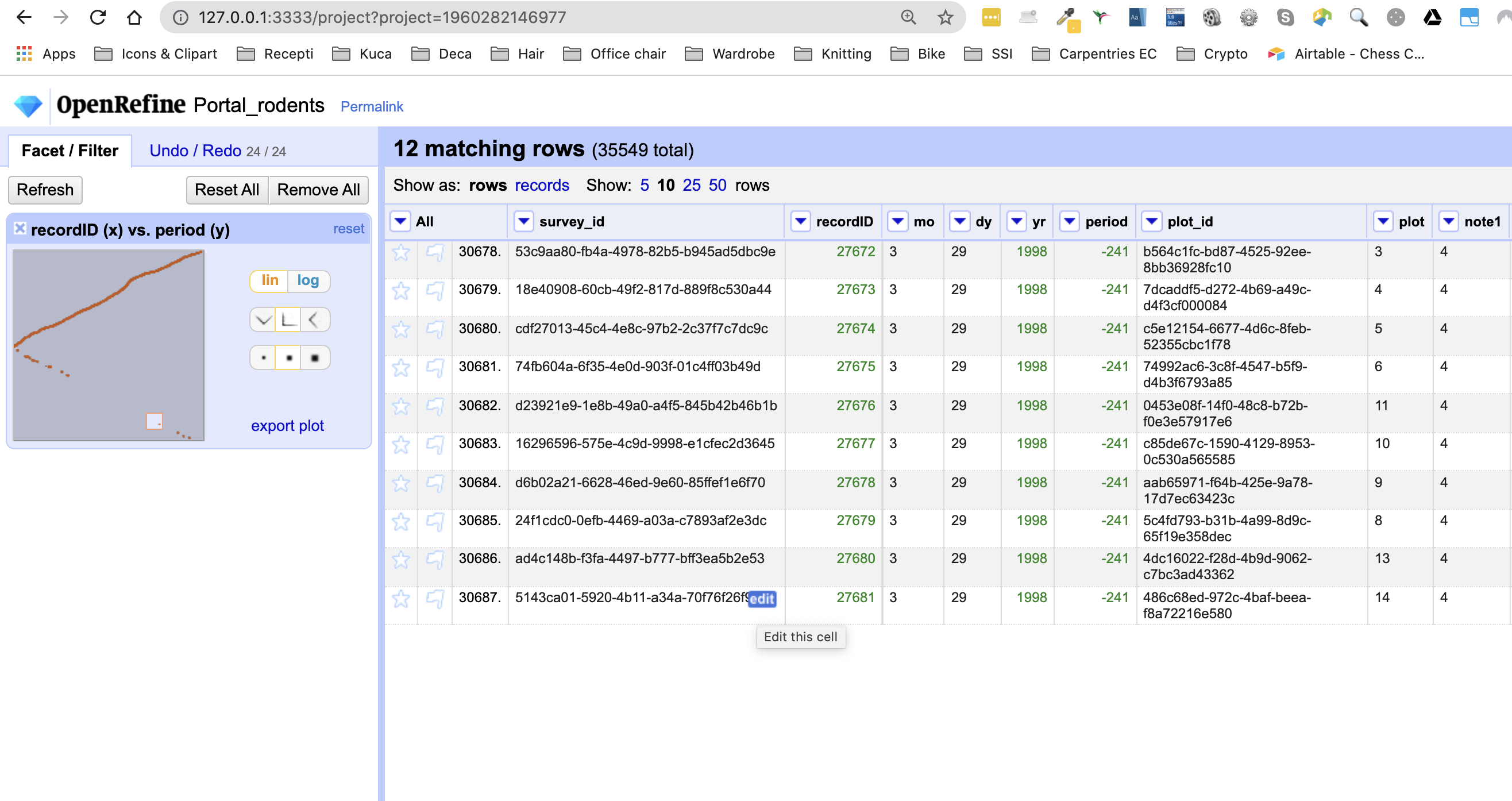
4. You can click in this panel to sort the facet by name and count. Do you notice any problems with the data? What are they?
5. Hover the mouse over any one of the names in the left panel. You should see that you have an edit function available.
6. You could use this to fix an error immediately, and OpenRefine will ask whether you want to make the same correction to every value equal to the one you identified. But OpenRefine offers even better ways to find and fix errors across the whole dataset, which we will use instead. We will learn about these when we talk about clustering.

There will be several near-identical entries in scientificName. For example, there is one entry for Ammospermophilis harrisi and one entry for Ammospermophilus harrisii. These are both misspellings of Ammospermophilus harrisi. We will see how to correct these misspelled and mistyped entries in a later exercise.

Exercise

1. Using faceting, find out how many years are represented in the census (via the yr column).

2. Is the column formatted as a number, date or text?

3. Which year has the most and which year has the least observations?

Solution

1. For the column yr do Facet > Text facet. A box will appear in the left panel showing that there are 26 unique entries in this column.
2. If you try to apply a Numeric facet on the same column, you may notice that it won’t work. This is because, by default, all columns in OpenRefine are formatted as text.
3. You can change the data format to numbers by selecting the down arrow next to the yr column name, selecting Edit cells > Common transforms > To number. Notice when this change was applied that the values in the column changed from black to green, and from left-justified to right-justified. If you now select Facet > Numeric facet on column yr, a new box is created that shows a histogram of the number of entries per year. Notice that the data is shown as a number, not a date.
4. You can also transform the column data type to be date by selecting Edit cells > Common transforms > To date. Note the program will assume all entries take place on 1st January of the year. You can now choose a Timeline facet. If you change the date to date data type, undo that action from the Undo/Redo tab to revert to the numeric data type before moving on to the next step. We will cover undoing/redoing actions in more detail shortly.
5. Click Sort by count in the Text facet box to order the counts numerically. The year with the most observations is 1997, and the year with the least is 1977.

Default data type

Be default, all data imported in OpenRefine is treated as text. You have to tell OpenRefine explicitly to treat columns differently via Edit cells > Common transforms, e.g. as numbers. If you change the data type - it will appear in green.

Facets for working with numbers

As we have seen in the previous exercise, when data is initially imported into OpenRefine, all the columns are treated as text values. We have seen that we can transform columns to other data types (e.g. number or date) using the Edit cells > Common transforms feature. Here we will experiment more with changing columns to numbers to see what additional capabilities this grants us.

Transform cells in the recordID column to numbers by clicking the down arrow for the column, then Edit cells > Common transforms… > To number. You will notice the recordID values change from left-justified to right-justified, and from black to green.

Exercise

Transform more columns, e.g. recordID and yr, from text to numbers. Can all columns be transformed to numbers?

Solution

To convert to number, a column must include only numerals (0-9). If you apply a number transformation to a column that does not meet this criterion (e.g. scientificName column), you might get an error and no data will be transformed (you can check this under the Undo / Redo tab: you will see the stage will be described Text transform on 0 cells.)

Facets for working with numbers, including numeric and scatterplot facets, display graphs instead of lists of values. These graphs include ‘drag and drop’ controls you can use to set a start and end range to filter the data displayed.

Numeric facet

Sometimes there are non-numeric values or blanks in a column which could represent errors in data entry. We can use OpenRefine to find them with a Numeric facet. Remove the facets we created previously before you proceed to gain more space.

1. For a column you have transformed to numbers, e.g. recordID, edit one or two cells and replace the numbers with text (such as abc) or with a blank (i.e. no space, number or text). To do so, hover over the cell you want to modify and an edit button will appear. Click on it and you will be able to modify the cell’s value. If you receive an error Not a valid number, try again and this time change the Data Type in the edit box to Text.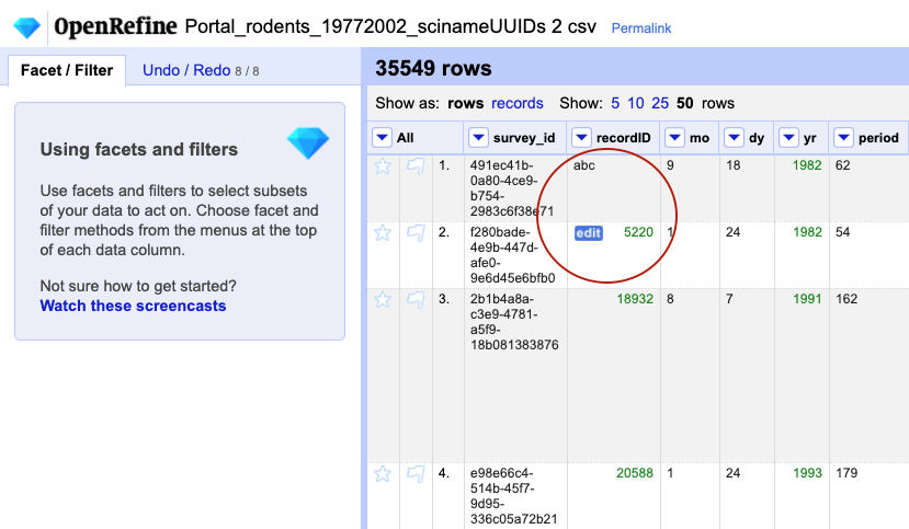

   

2. Now use the drop down menu next to the column name, select Facet > Numeric facet to apply a numeric facet to the column you edited. The graph representing the numeric facet will appear in the left panel.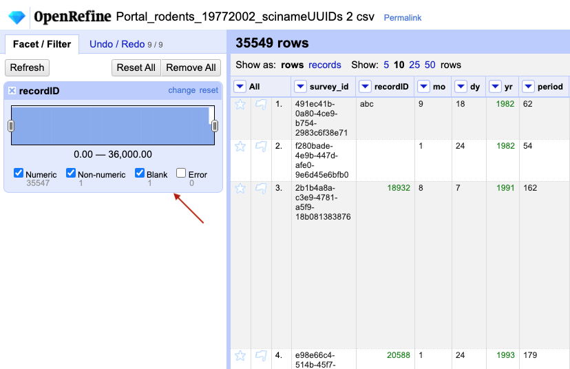

   

3. Notice that there are several checkboxes in this facet: Numeric, Non-numeric, Blank, and Error. Below these are counts showing the number of matching cells in each category. You should see checks for Non-numeric and Blank if you changed some values.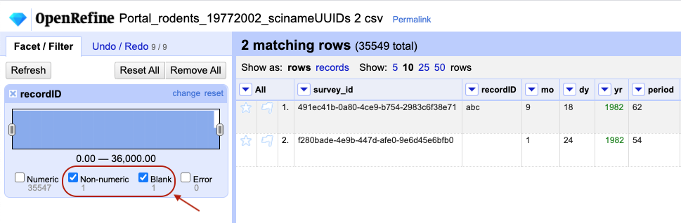

   

4. Experiment with checking or unchecking these boxes, and notice how this affects your data table.

When you have finished examining the numeric data, remove this facet by clicking the x in the upper left corner of its panel. Note that this does not undo the edits you made to the cells in this column. If you want to reverse these edits, use the Undo / Redo function.

Scatterplot facet

Now that we have multiple columns representing numbers, we can see how they relate to one another using the scatterplot facet.

Select a numeric column, for example recordID, and use the pulldown menu to > Facet > Scatterplot facet. A new window called Scatterplot Matrix will appear. It contains grids for each pair of numeric columns that have been plotted against each other (the number will vary dependent on how many columns you have transformed to numbers).

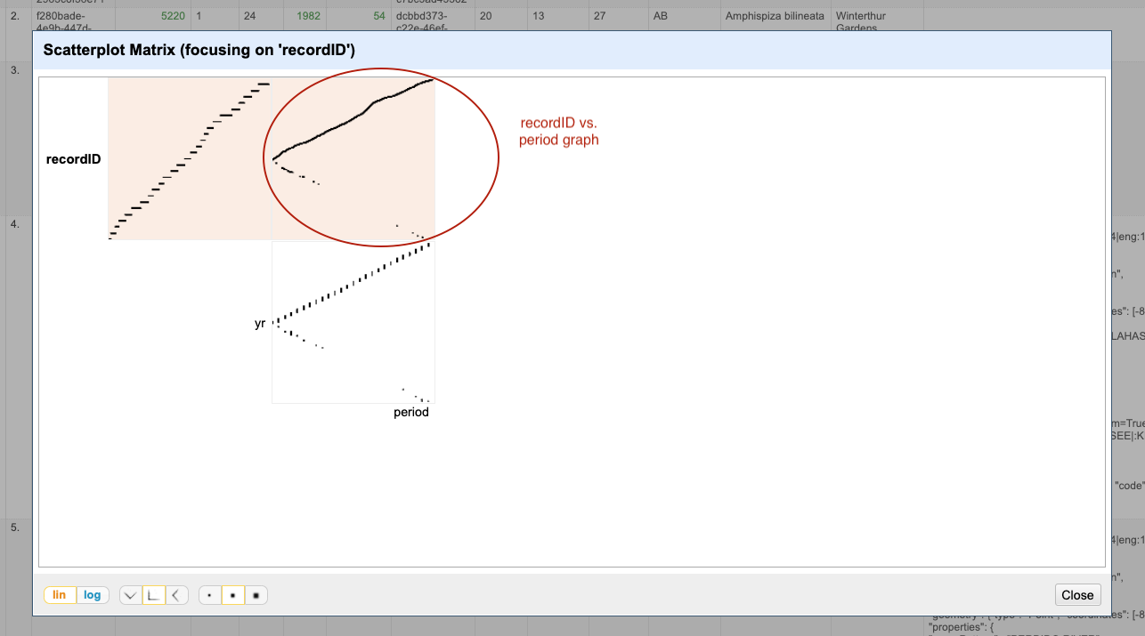
1. Examine the scatterplots overall. Do the patterns make sense?
2. Why does the scatterplot for recordID vs period have the pattern it does?

We can examine one pair of columns by clicking on its square in the Scatterplot Matrix A new facet with only that pair of columns will appear in the left margin as an interactive graph. Click in the scatterplot facet in the left margin and drag to highlight a rectangle. This is a very powerful way of subsetting data of interest.

The scatterplot recordID vs period has a slightly unexpected shape - you would probably expect a linear graph. Instead, there are some negative values on the period axis. These are potentially errors in the data. You can click anywhere on the graph to get rid of the subsetting.

Other types of facets

In addition to Text, Numeric, Scatterplot and Timeline facets, OpenRefine also supports a range of customized facets:

• Word facet - this breaks down text into words and counts the number of records in which each word appears
• Duplicates facet - this results in a binary facet of ‘true’ or ‘false’. Rows appear in the ‘true’ facet if the value in the selected column is an exact match for a value in the same column in another row
• Text length facet - creates a numeric facet based on the length (number of characters) of the text in each row for the selected column. This can be useful for spotting incorrect or unusual data in a field where specific lengths are expected (e.g. if the values are expected to be years, any row with a text length more than 4 for that column is likely to be incorrect)
• Facet by blank - a binary facet of ‘true’ or ‘false’. Rows appear in the ‘true’ facet if they have no data present in that column. This is useful when looking for rows missing key data.

Facets are used to group together common values. OpenRefine limits the number of values allowed in a single facet to ensure the software does not perform slowly or run out of memory. If you create a facet where there are many unique values (for example, a facet on a ‘book title’ column in a data set that has one row per book) the facet created will be very large and may either slow down the application, or OpenRefine will refuse to create the facet.

Key Points

• Faceting can identify errors or outliers in data.

Transforming Data

Overview

Teaching: 30 min
Exercises: 10 min

Questions

• How can we transform our data to correct errors?

Objectives

• Learn about clustering and how it is applied to group and edit typos.

• Split values from one column into multiple columns.

• Manipulate data using previous cleaning steps with undo/redo.

• Remove leading and trailing white spaces from cells.

• Learn to use GREL (General Refine Expression Language) for advanced data transformations.

So far we have learned to use various facets to inspect and explore our data. Text facet also allowed us to directly edit a subset of data in bulk. We have also seen how we can transform the data type from text to numeric. OpenRefine offers a number of other functionalities to transform and restructure the data.

Data clustering

Clustering allows you to find groups of entries that are are not identical but are sufficiently similar that they may be alternative representations of the same thing (term or data value). For example, the two strings New York and new york are very likely to refer to the same concept and just have a capitalisation differences. Likewise, Björk and Bjork probably refer to the same person. These kinds of variations occur a lot in scientific data. Clustering gives us a tool to resolve them.

OpenRefine provides different clustering algorithms. The best way to understand how they work is to experiment with them.

1. If you removed it, reinstate the scientificName text facet (you can also remove all the other facets to gain some space). In the scientificName text facet box - click the Cluster button.
2. In the resulting pop-up window, you can change the Method and the Keying Function. Try different combinations to see what different mergers of values are suggested.

3. If you select the key collision method and the metaphone3 keying function. It should identify three clusters.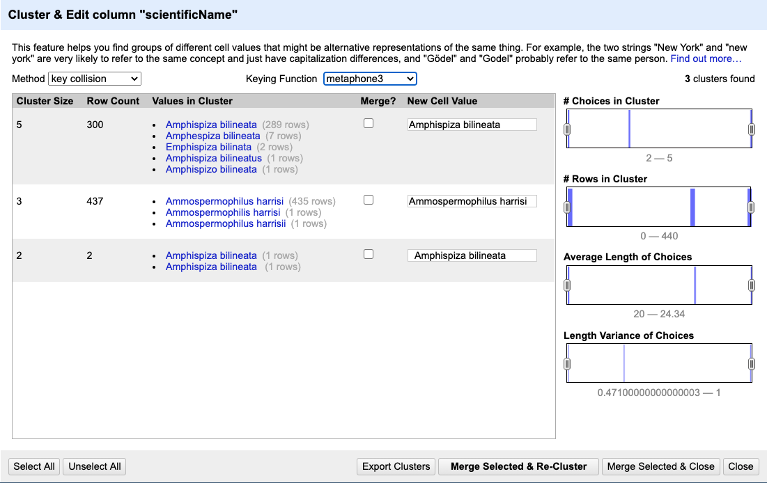

   

4. Tick the Merge? checkbox beside each group, then click Merge Selected and Recluster to apply the corrections to the dataset. Note that the New Cell Value column displays the new name that will replace the value in all the cells in the group. You can change this (but please don’t do so now) if you wish to choose a different value than the suggested one.
5. Try selecting different Methods and Keying Functions again, to see what new merges are suggested. You may find there are still improvements that can be made, but do not Merge again; just Close when you are done. We will now see other operations that will help us detect and correct the remaining problems, and that have other, more general uses.

Important: If you Merge using a different method or keying function, or more times than described in the instructions above, your solutions for later exercises will not be the same as shown in those exercise solutions.

OpenRefine Wiki: Clustering

Full documentation on clustering can be found at OpenRefine Wiki: Clustering

Data splitting

It is easy to split data from one column into multiple columns if the parts are separated by a common separator (say a comma, or a space).

1. Let us suppose we want to split the scientificName column into separate columns, one for genus and one for species.
2. Click the down arrow next to the scientificName column. Choose Edit Column > Split into several columns...
3. In the pop-up, in the Separator box, replace the comma with a space (the box will look empty when you’re done).
4. Important! Uncheck the box that says Remove this column.
5. Click OK. You should get some new columns called scientificName 1, scientificName 2, scientificName 3, and scientificName 4.
6. Notice that in some cases these newly created columns are empty (you can check by text faceting the column). Why? What do you think we can do to fix it?

The entries that have data in scientificName 3 and scientificName 4 but not the first two scientificName columns had an extra space at the beginning of the entry. Leading and trailing white spaces are very difficult to notice when cleaning data manually. This is another advantage of using OpenRefine to clean your data - this process can be automated. In newer versions of OpenRefine (from version 3.4.1) there is now an option to clean leading and trailing white spaces from all data when importing the data initially and creating the project. Because we didn’t clean white space at the time of importing the data, we will look at how to fix leading and trailing white spaces manually in a moment - first we need to undo the splitting step.

Undoing / Redoing actions

It is common while exploring and cleaning a dataset to make a mistake or decide to change the order of the process you wish to conduct. OpenRefine provides Undo and Redo operations to make it easy to roll back your changes.

1. Click Undo / Redo in the left side of the screen. All the changes you have made will appear in the left-hand panel. The current stage in the data processing is highlighted in blue (i.e. step 4. in the screenshot below). As you click on the different stages in the process, the step identified in blue will change and, far more importantly, the data will revert to that stage in the processing.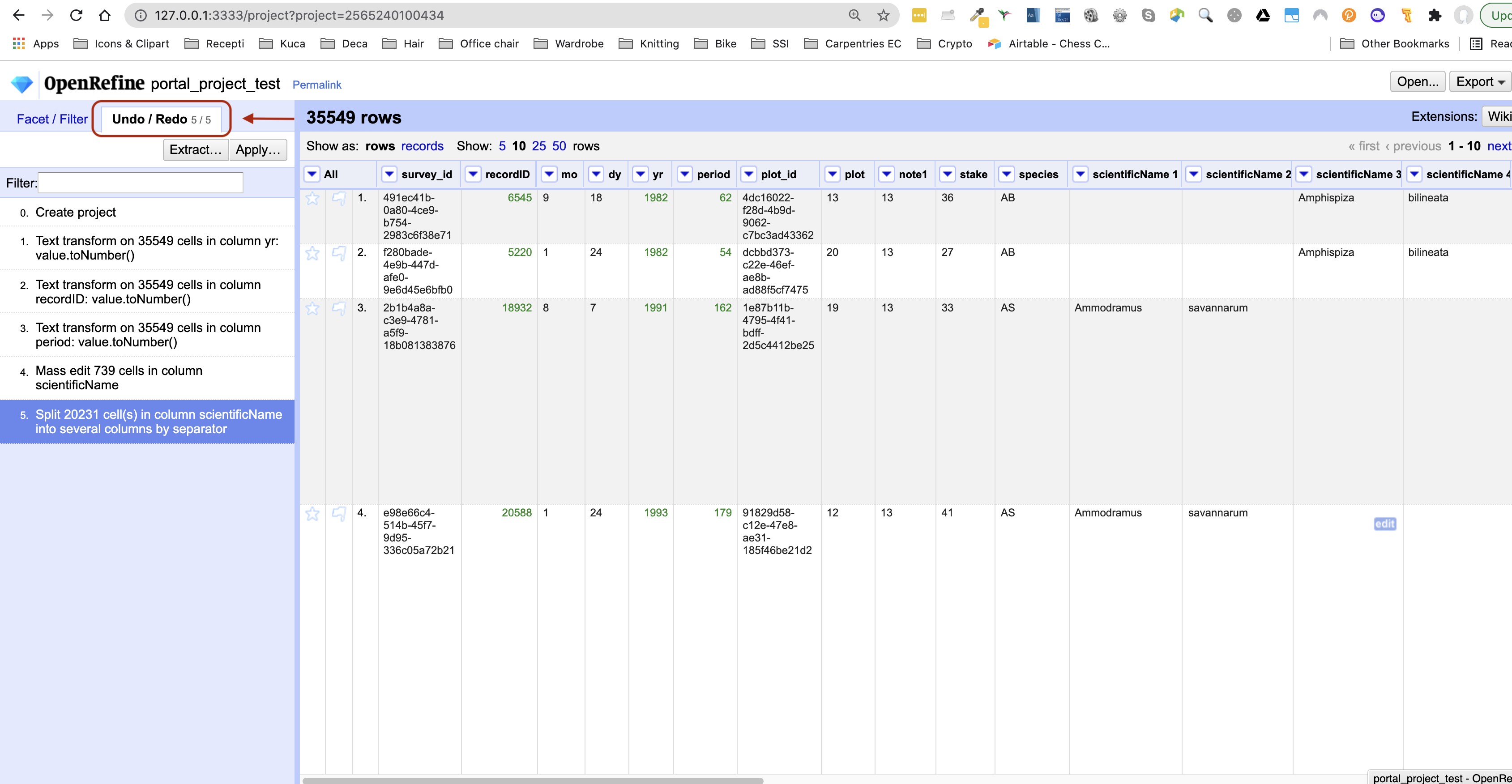

   

2. We want to undo the splitting of the column scientificName. Select the stage just before the split occurred and the new scientificName columns will disappear.
3. Notice that you can still click on the last stage and make the columns reappear, and toggle back and forth between these states. You can also select the state more than one steps back and revert to that state.
4. Let’s leave the dataset in the state in which the scientificNames were clustered, by selecting the stage just before the split.

Important: If you skip this step, your solutions for later exercises will not be the same as shown in those exercise solutions.

Trimming Leading and Trailing Whitespace

Words with spaces at the beginning or end are particularly hard for humans to identify from strings without these spaces (as we have seen with the scientificName column). However, blank spaces can make a big difference to computers, so we usually want to remove them.

1. In the header for the column scientificName, choose Edit cells > Common transforms > Trim leading and trailing whitespace.
2. Notice that the Split step has now disappeared from the Undo / Redo pane on the left and is replaced with a Text transform on 3 cells
3. Perform the same Split operation on scientificName that you undid earlier. This time you should now only get two new columns.

Removing the leading white spaces means that each entry in this column has exactly one space (between the genus and species parts of the original scientificName data). Therefore, when you now split with space as the separator, you should get only two columns. Let’s do this as an exercise.

Exercise

Repeat the splitting of column scientificName exercise.

Solution

On the scientificName column, click the down arrow next to the scientificName column and choose Edit Column > Split into several columns... from the drop down menu. Use a blank character as a separator, as before. You should now get only two columns scientificName 1 and scientificName 2.

Renaming columns

We now have the genus and species parts neatly separated into 2 columns - scientificName 1 and scientificName 2. We want to rename these as genus and species, respectively.

1. Let’s first rename the scientificName 1 column. On the column, click the down arrow and then Edit column > Rename this column.
2. Type “genus” into the box that appears.

Exercise

Try to change the name of the scientificName 2 column to species. What problem do you encounter? How can you fix the problem?

Solution

1. On the scientificName 2 column, click the down arrow and then Edit column > Rename this column.
2. Type “species” into the box that appears.
3. A pop-up will appear that says Another column already named species. This is because there is another column with the same name where we’ve recorded the species abbreviation.
4. You can choose another name like speciesName for this column or change the other species column name to species_abbreviation and then come back and rename this column to species.

Important: Undo the splitting and renaming steps and retain the white space trimming step before moving on (it may be several steps back). If you skip this step, your solutions for later exercises will not be the same as shown in exercise solutions.

Transforming Data Using GREL

OpenRefine provides a way to write special expressions to accomplish more complex data transformations (such as string manipulation or mathematical calculations) to improve the structure of the data. These functions are written in a special language called GREL (General Refine Expression Language). GREL can be used in several places:

1. when transforming cells in a column using the transformation function
2. when adding a column based on another column
3. when creating a custom Text or Numeric facet
4. when creating a new column by fetching data from a URL

We will have a look at the first two of these options; you can explore other yourself - the principle of using GREL will be the same and all GREL input windows in OpenRefine will have a very similar outlook.

Let’s have a look at the column geolocation - it contains latitude and longitude coordinates of locations where observations took place combined together like this: ('30.438056', '-84.247155'). As can be noted, data contains round braces “(“ and “)” and single quotes “’” around data making it less useful for any processing. We want to get rid of all these characters and split the data in two columns to contain individual values for latitude and longitude.

1. First we want to create a duplicate of the geolocation column where we will perform our operations and keep the original geolocation intact. To do so, on the geolocation column click the down arrow and then Edit column > Add column based on this column....

2. You will be presented with a window to enter a GREL expression telling OpenRefine how to transform the current data when creating a new column based off it.

   

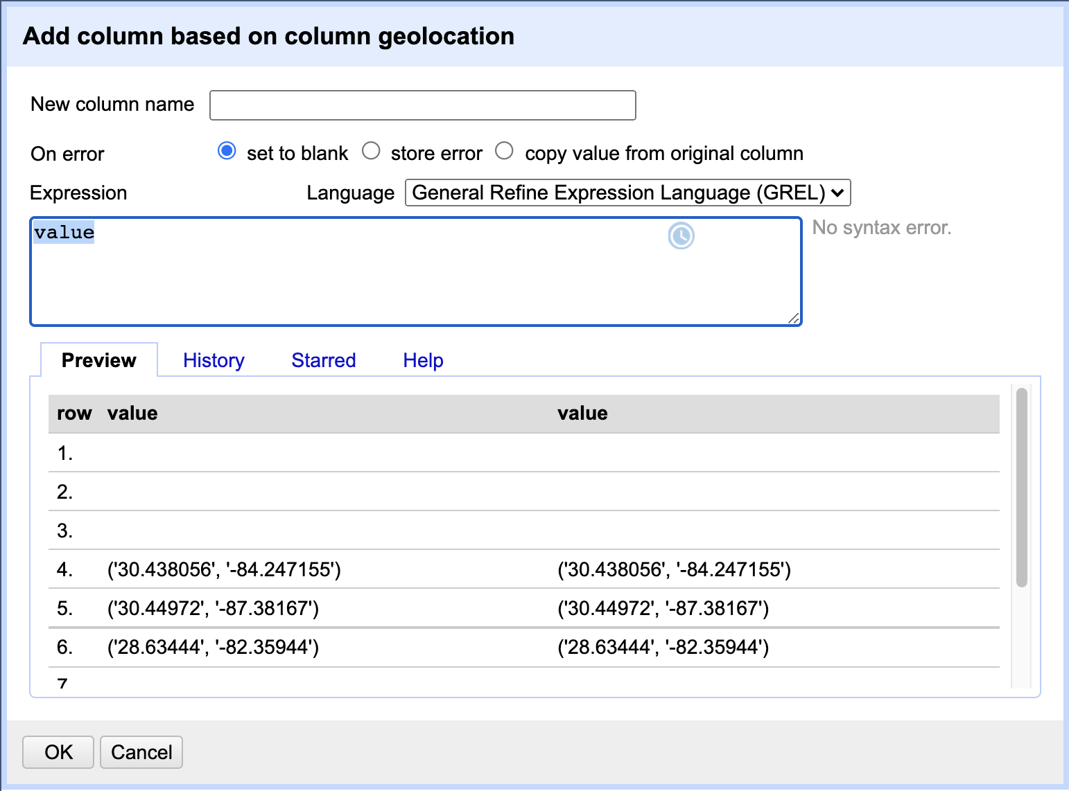
   GREL Expression field contains the expression “value” to begin with. This indicates to use the current “value” of the cell as is when transforming data. In the Preview panel below you can also see the current cell value and what the new value would be after applying the GREL expression to it (in this case - both values will be the same as we are simply duplicating the column). In the New column name field type the new new name for our duplicate column, e.g. geolocation_new. When finished, click OK to apply the action.

3. After OpenRefine creates the geolocation_new column, we want to do further transformations on it to extract longitude and latitude values. To do so, select Edit cells > Transform... from the drop down menu on the geolocation_new column. You will once again be presented with a similar window to enter a GREL expression. This time, we want to chain a few functions in the GREL expression to achieve the desired effect of removing round braces and single quotes, like so: value.replace("(","").replace(")","").replace("'",""). We are replacing any occurrence of “(“ in the cell data value with a blank character (effectively deleting it), and then repeating (chaining) similar functions on the output value from the previous function until we remove all unwanted characters. Try typing one function at a time to see what effect it has on the data - you can see the result of applying each expression in the Preview panel.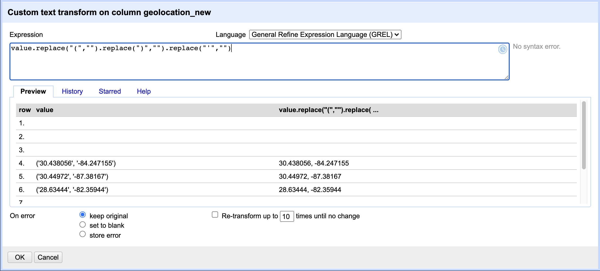

   

   When finished, click OK to apply the data transformation.

4. We are now ready to split the geolocation_new column using the Edit Column > Split into several columns..., as we learned earlier in this episode. The separator we want to use in this case is “, “ - a comma followed by a blank character. If, in addition, you select the Guess cell type checkbox in the split column popup window, OpenRefine will correctly identify that the values in new columns are numeric and transform the data type for us as well.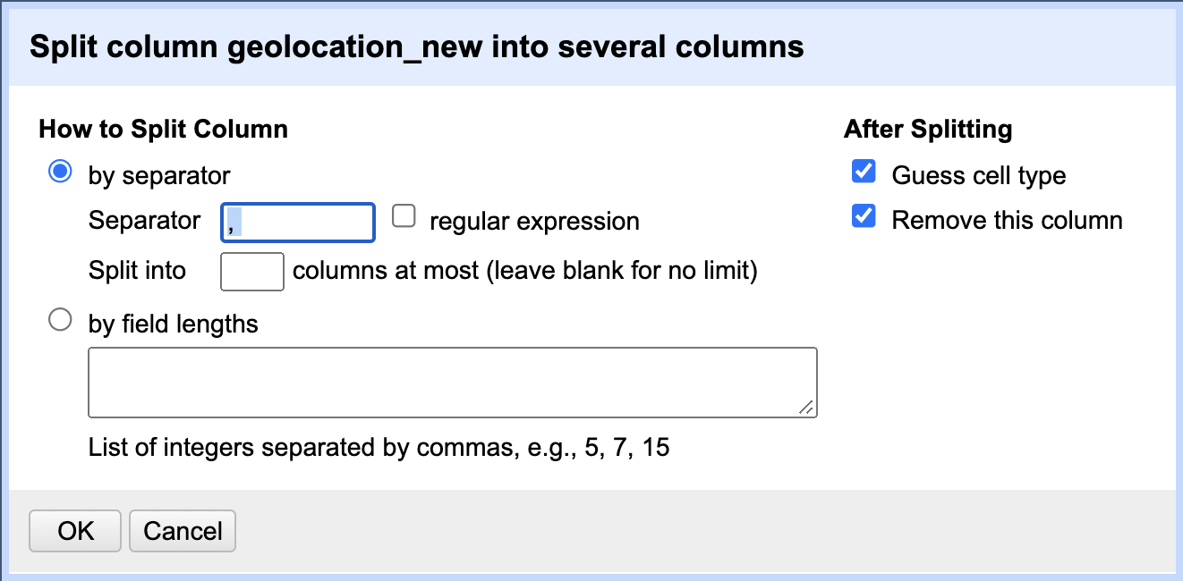

   

5. You should now have 2 new columns with numeric data named geolocation_new 1 and geolocation_new 2 representing the extracted longitude and latitude values respectively.
6. Rename your new columns to longitude and latitude accordingly. You can now make further use of the extracted data from other applications, e.g. plot geolocations on a map.

GREL offers rich syntax and a large number of functions for complex string manipulations (and handling different text formats - JSON, HTML, XML), working with numbers, dates and boolean (TRUE/FALSE) values, logical and mathematical operations. We strongly recommend learning more on GREL syntax and functionalities.

GREL documentation

Check the official GREL documentation for the full reference on GREL. Here is another useful GREL guide to check out.

Key Points

• Clustering can identify outliers in data and help us fix errors in bulk.

• GREL (General Refine Expression Language) is a powerful tool for transforming data.

Filtering and Sorting Data

Overview

Teaching: 20 min
Exercises: 10 min

Questions

• How can we select only a subset of our data to work with?

• How can we sort our data?

Objectives

• Employ text filters or sub-setting options in facets to filter to a subset of rows.

• Sort data by one or multiple columns.

Filtering data

Sometimes you want to view and work only with a subset of data or apply an operation only to a subset. You can do this by applying various filters to your data.

Including/excluding data entries on facets

One way to filter down our data is to use the include or exclude buttons on the entries in a text facet. If you still have your text facet for scientificName, you can use it. If you’ve closed that facet, recreate it by selecting Facet > Text facet on the scientificName column.

1. In the text facet, hover over one of the names, e.g. Baiomys taylori. Notice that when you hover over it, there are buttons to the right for edit and include.
2. Whilst hovering over Baiomys taylori, move to the right and click the include option. This will include this species, as signified by the name of the species changing from blue to orange, and new options of edit and exclude will be presented. Note that in the top of the page, “46 matching rows” is now displayed instead of “35549 rows”.
3. You can include other species in your current filter - e.g. click onChaetodipus baileyi in the same way to include it in the filter.
4. Alternatively, you can click the name of the species to include it in the filter instead of clicking the include/exclude buttons. This will include the selected species and exclude all others options in a single step, which can be useful.
5. Click include and exclude on the other species and notice how the entries appear and disappear from the data table to the right.

You can also filter data using other types of facets - let’s do it as an exercise.

Exercise

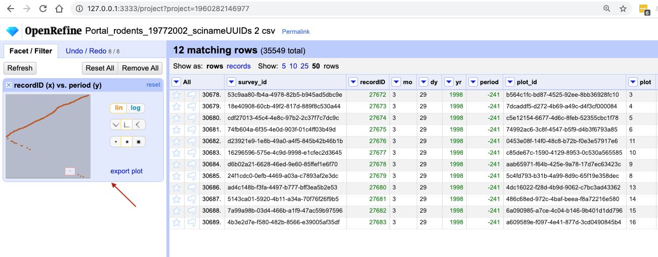
Remove all current facets and recreate the scatterplot facet for recordID and period columns as before. Drag a rectangular selection anywhere on the Scatterplot Matrix square for recordID and period. Notice how the filtered data change to show only entries included in the rectangle.

Solution

In the screenshot below, we have filtered out only 12 entries by dragging a small rectangular selection on the scatterplot graph. As before, when we first introduced the scatterplot facet, we can notice that something is potentially wrong with our data as values for period in the filtered subset are negative (we are expecting only positive values) and potentially require futher examination and cleaning.

Text filters

Another way to filter data is to create a text filter on a column. Close all facets you may have created previously and reinstate the text facet on the scientificName column.

1. Click the down arrow next to scientificName > Text filter. A scientificName filter will appear on the left margin below the text facet.

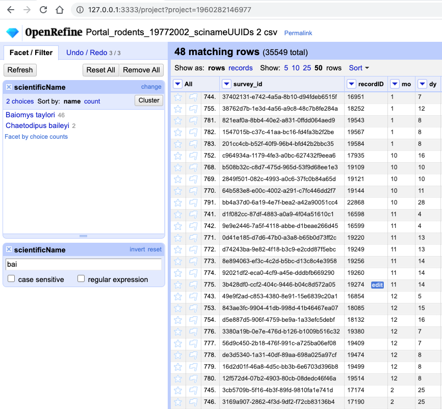
2. Type in bai into the text box in the filter and press return. At the top of the page it will report that, out of the 35549 rows in the raw data, there are 48 rows in which the text has been found within the scientificName column (and these rows will be selected for the subsequent steps).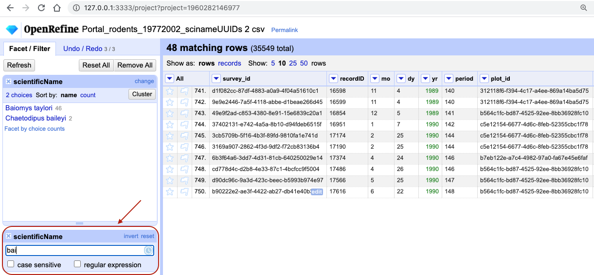

   

3. Near the top of the screen, change Show: to 50. This way, you will see all the matching rows in a single page.

Exercise

1. What scientific names are selected by this text filter?
2. How would you restrict it to one of the species selected?

Solution

1. If you kept a text facet over scientificName from before - it will show that two names match your filter criteria are: Baiomys taylori and Chaetodipus baileyi. If you have closed the text facet, select Facet > Text facet on the scientificName column to reinstate it.
2. There are various options to restrict to only one of the two species identified. You could make the search case sensitive. You could split the scientificName column into species and genus columns, as before, and filter only the column of interest. You could include more letters in your filter, e.g. baio which would exclude Chaetodipus baileyi. Try playing with these different options. You could include more letters in your filter, e.g. baio which would exclude Chaetodipus baileyi. Try playing with these different options.

Important: Make sure both species are included in your filtered dataset before continuing with the rest of the exercises.

Filters vs. facets

Faceting and filtering look very similar. A good distinction is that faceting gives you an overview of all the data that is currently selected, while filtering allows you to select a subset of your data for further inspection and analysis.

Sorting data

Sorting data is a useful practice for detecting outliers in data - potential errors and blanks will sort to the top or the bottom of your data.

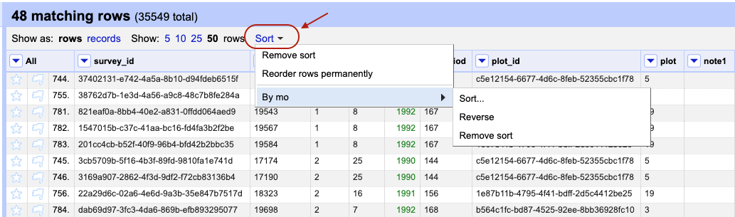
To sort the data in a column, click the arrow next to your chosen column name and select Sort.... This will open a pop-up that will present you with different options, e.g. whether you wish to sort by text, numbers, dates or booleans (i.e. TRUE or FALSE values). Additional options will appear to allow you to fine-tune your sorting - e.g. you can specify where to place Blanks and Errors in the sorted results.

Exercise

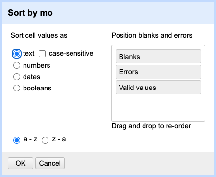
Try sorting the data by month using the column mo. What happens if you sort the column as text? How can you ensure that months are in order?

Solution

From the drop-down menu on the column mo select Sort then Sort.... Select Sort cell values as text first. (Note that you can rearrange Errors, Blanks and Valid values so that errors and blanks will sort to the top. This is a good practice detect some outliers.)

You will notice that values for month have been sorted in alphabetical order, where months 10, 11 and 12 came before month > > 2.

This is probably not what you wanted - so you will have to redo the sort and select the Sort cell values as number option.

You may have noticed that in the case of sorting as numbers, the actual column itself remained as text. OpenRefine did not convert the column to numbers (notice the absence of the green font).

Another thing to note is that sorting is not an action that you can undo/redo - it does not appear on Undo/Redo tab. This is because sorting only rearranges the order of the data, it doesn’t change its content. This means the sorting will not change the cells in a column from text to numbers - rather, it will interpret the values as numbers for the purposes of sorting, but will keep the underlying data type unchanged.

The first time you sort a column, the first option will present as Sort.... If you re-sort a column that you have already sorted, the drop-down menu changes slightly: the first option will be Sort and the following sub-options will be presented:

• Sort... - This option enables you to choose a new sort.
• Reverse - This option allows you to reverse the order of the sort.
• Remove sort - This option allows you to undo your sort.

It may not always be that obvious in OpenRefine that you performed a sort. Once you complete the sort for the first time a Sort button will appear at the top of the page as an indicator that the data has been sorted. It will disappear if you remove the sort.

Exercise

Remove the sort by month. Make sure you still have the text filter for the text “bai” on the scientificName column present (if you have lost your text filter for “bai” see the start of the episode to help you reinstate it). Then sort the data by plot. In which year(s) were observations recorded for plot 1 in the filtered dataset?

Solution

From the drop-down menu on the column plot select Sort... then Sort cell values as numbers and smallest first. The years observations were recorded in plot 1 are 1990 and 1995.

Sorting by multiple columns

Once you have completed one sort, any further sort will be performed by default as an additional sort. For example, if you take the data that has been sorted by plot and the sort by year, OpenRefine will present the data sorted by plot and then by year. If you wish to restart the sorting process, check the sort by this column alone box in the Sort pop-up menu.

Exercise

You might like to look for trends in your data by month of collection across years.

1. How do you sort your data by month?
2. How would you do this differently if you were instead trying to see all of your entries in chronological order?

Solution

1. To sort by month, click on Sort... from the mo column, and then select Sort cell values as numbers. This will group all entries made in, for example, January, together, regardless of which year that entry was collected.
2. To sort chronologically, click on Sort > Sort... from the yr column , and then select Sort cell values as numbers. Before clicking ‘OK’ make sure you select sort by this column alone to start a new sort from scratch.
3. You can now apply an additional sort, this time by month (click on Sort from the mo column, and then select Sort cell values as numbers).
4. To ensure that all entries are shown chronologically, you will need to add a third sorting step to sort data by day (using the column dy).

If you go back to one of the already sorted columns and select Sort > Remove sort, that column is removed from your multiple sort. If it is the only column sorted, then the data revert to their original order.

Exercise

Sort by year, month and day in some order. Be creative: try sorting as numbers or text, and in reverse order (largest to smallest or z to a).

Use Sort > Remove sort to remove the sort on the second of three columns. Notice how that changes the order.

Sorting does not change data

You may have noticed that after any of the sorting steps there was nothing to undo/redo. This is because you have only reordered and not modified you data. If you want to revert to the original order of the data - make sure you remove all “sorts” using the Sort > Remove sort option.

Key Points

• OpenRefine provides various ways to sort and filter data without affecting the raw data.

Exporting Data Cleaning Steps

Overview

Teaching: 10 min
Exercises: 5 min

Questions

• How can we document the data-cleaning steps we’ve applied to our data?

• How can we apply these steps to additional data sets?

Objectives

• Describe how OpenRefine generates JSON code.

• Demonstrate ability to export JSON code from OpenRefine.

• Save JSON code from an analysis.

• Apply saved JSON code to an analysis.

Scripts

We have seen that from the section on Undo / Redo that OpenRefine saves every change you make to the dataset. You can export this information so that you can apply the same process to other datasets without having to go through each of the individual steps. This saves a lot of time, because you frequently will apply the same data cleaning steps to a number of datasets over time. The files must all had the same structure, the same type of errors (e.g. species name misspellings, leading white spaces) and the same column names.

The information about the transformations that have taken place are stored in OpenRefine using a format known as JSON (JavaScript Object Notation). This is a popular, open standard for data interchange that benefits from also being human readable (you may not believe this, but it’s certainly more readable than most).

You’re going to need a tool to save the JSON during this next exercise. Any text editor will work (like NotePad on Windows or TextEdit on Mac). Do not use a Word Processor (e.g. Word) for this step, because they have a tendency to automatically change text for perceived grammatical or spelling mistakes. This will, of course, render the JSON useless.

1. In the Undo / Redo section, click Extract... in the top left corner of the screen
2. A pop up will open which includes two columns: one lists the steps you have taken to transform your data with tick boxes next to each step, and the other lists same information in the JSON format (this is a text file peppered with lots of {, :, , and ")
3. As you check and uncheck the tick boxes, the JSON will change appropriately. For now, ensure that all tick boxes are ticked so that all the steps are selected.
4. Highlight all of the JSON from the right hand panel and then copy it.
5. Paste the JSON into your text editor (see above for details), then save it as a plain text file, i.e. .txt. In TextEdit, do this by selecting Format > Make plain text and save the file as a my_analysis.txt.

In practice, you would re-run the steps on a new dataset, but to keep things simple, in the next example we will re-run the steps on the original dataset.

1. Start a new project in OpenRefine: click the “OpenRefine” name in the top-left hand corner of the screen to be taken back to the main interface. Create a project using the same dataset as last time (if you’ve misplaced it, you can download a new copy)
2. Once the dataset has loaded, click the Undo / Redo tab then the Apply button.
3. A pop-up will open with a blank text filed into which you can paste the JSON contents of your my_analysis.txt file.
4. Click Perform operations. The pop up will close, and all of the transformations you applied to the previous dataset will be re-applied to your current dataset to produce a new cleaned dataset.

Although this process only involved the re-application of 5 or 6 steps, with real research data you could be reapplying hundreds of transformations - and you might have to re-apply those steps to tens of datasets. This is why there is such potential for saving time with the export/apply functionality of OpenRefine.

Reproducible science

Now, that you know how scripts work, you may wonder how to use them in your own scientific research. For inspiration, you can read more about the successful application of the reproducible science principles in archaeology or marine ecology:

1. Marwick et al. (2017) Computational Reproducibility in Archaeological Research: Basic Principles and a Case Study of Their Implementation
2. Stewart Lowndes et al. (2017) Our path to better science in less time using open data science tools

Key Points

• All changes are being tracked in OpenRefine (apart from individual cell changes and sorting!), and this information can be used for scripts for future analyses or reproducing an analysis.

• Scripts can (and should) be published together with the dataset as part of the digital appendix of the research output.

Exporting and Saving Data

Overview

Teaching: 10 min
Exercises: 5 min

Questions

• How can we save and export our cleaned data from OpenRefine?

Objectives

• Save an OpenRefine project.

• Export cleaned data from an OpenRefine project.

OpenRefine saves your project as you work automatically, so you don’t need to worry about saving. It saves projects in a slightly obscure and hidden location (check where OpenRefine stores project data for different operating systems), most likely to prevent users from accidentally tempering with them. You can, however, export the “OpenRefine project” in a location of your choice, which will package together the data and all the information about the cleaning and data transformation steps you’ve performed. You can then use the exported project to transfer your work to another computer, share the project with collaborators, archive it with your research, etc.

Exporting a project

1. Click the Export button in the top right and select OpenRefine project archive to file. You might be moved to a new blank tab in your browser might whilst this function is executing.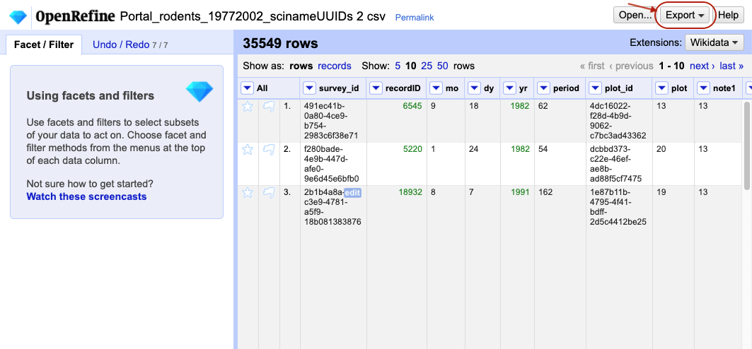

   

2. A .tar.gz file will download to your default Download directory. The tar.gz extension tells you that this is a compressed file, which means that it contains multiple files (the most common version of this file type is .zip which you may be aware of).
3. You can share the .tar.gz file with collaborators, or copy it to a different computer and import the project back into OpenRefine (say, to do further work at home). Note: sharing of this type is best performed via version control software, such as Git.

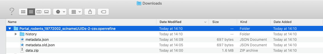
If you wish to investigate the files, you can double-click on the tar.gz file and it will expand into a directory (this process can be more complicated in Windows - see below for details). A folder icon will now appear. Investigate the files in this folder. What files appear? What information do you think they contain?

Opening a .tar.gz file on Windows:

• You may require additional software such as 7-zip or WinZip. Download and run the installer of your choice.
• Double-click the exported tar.gz file. If Windows asks how you want to open the file, check the “Always use this app to open .gz files” box, then select “More apps”.
• If your chosen application is not listed, select ‘Look for another app on this PC’.
• In the file browser, navigate to C:\Program Files, find the application you installed, and double-click on its executable (7zFM, for example).

Once you open the .tar.gz OpenRefine project fine, you should see:

• a history folder which contains three zip files. Each of these contains a change.txt file, which lists each of the individual transformation that you performed on your data.
• a data.zip file. When expanded, this zip file includes a file called data.txt which is a copy of your raw data. You may also see other files.

Importing a new project

You can import an exported project into OpenRefine as follows:

1. Click Open... in the top-right of the screen, which will take you back to OpenRefine’s main interface.
2. Select Import Project from the left-hand panel and, click Choose files and navigate to the .tar.gz file in the window that opens. Click the file and select Open (or just double-click the file).
3. The project will open. It include all of the raw data and the cleaning steps that were part of the original project.

Opening an existing project

When you open OpenRefine (or navigate to http://localhost:3333/ from an already open project), you will see a list of projects already saved on your machine that you have created or imported earlier. You can click on any one of them to open them and continue working on them in OpenRefine.

Exporting Cleaned Data

You can also export just your cleaned data from an OpenRefine project (as opposed to the whole project), if you wish to save it in a form more suited to further analysis (e.g. as CSV) and so that it can be used by other programs. For example, you might wish to save the data into a .csv file so that you can conduct further analysis using Python or R.

1. Click Export in the top right and select the file type you want to export
   • Comma-separated values (csv) is a good choice, because it’s a file type that can be read by most other data analysis programs. Tab-separated values (tsv) is also a popular format.
2. The cleaned data will be exported to your default Download directory.

Using widely-supported, open, static and non-proprietary file formats like .csv or .tsv make it easier for yourself and others to use your data in the future.

Key Points

• Cleaned data or entire projects can be exported from OpenRefine.

• Projects can be shared with collaborators, enabling them to see, reproduce and check all data cleaning steps you performed.

Further Resources on OpenRefine

Overview

Teaching: 5 min
Exercises: 0 min

Questions

• What other resources are available for working with OpenRefine?

Objectives

• Explore the online resources available for more information on OpenRefine.

• Identify other resources about OpenRefine.

OpenRefine resources

OpenRefine is more than a simple data cleaning tool. People are using it for all sorts of activities. Here are some other resources that might prove useful.

OpenRefine has its own website with documentation and a book:

• OpenRefine web site
• OpenRefine Documentation for Users (Wiki site)
• Using OpenRefine book by Ruben Verborgh, Max De Wilde and Aniket Sawant
• OpenRefine history from Wikipedia

In addition, see these other useful resources:

• Grateful Data is a fun site with many resources devoted to OpenRefine, including a nice tutorial.
• Margaret Heller shows how she uses OpenRefine for Measuring and Counting Impact in Repositories.
• Intersect Course Resources contains Jared Berghold’s ‘Cleaning & Exploring your data with Open Refine’.

There are more advanced uses of OpenRefine, such as bringing in column or cell data using web locators (URLs or APIs). The links above can give you a start on your journey.

Key Points

• Other examples and resources online are good for learning more about OpenRefine

Survey

Overview

Teaching: min
Exercises: min

Questions

Objectives

Post-Lesson Survey

Key Points